Optimizing Chemical Processes
Dr. Patrick Bangert
algorithmica technologies GmbH
A chemical plant’s efficiency and profitability can be optimized using mathematical modeling. The optimization tells plant operators which set-points should be changed to obtain the maximum profitability.This method requires no engineering changes to be made to the plant. We show that a profitability increase of approximately 6% was possible in a specific chemical plant producing silanes, with an overall yield increase of 5.1% and an increase of 2.9% for the most profitable end product.
Like other industries, the chemical industry constantly aims to enhance the profitability of its plants by increasing the production yield.Such increase may be achieved either via engineering changes, which arequite cost intensive, or via operational changes. Operational changes can increase yield and profitability without actually changing the equipment and the processes of the plant.The question is: What operational changes are needed to increase yield, or better still, to optimize yield under the given circumstances? Here, we compute the action required to achieve optimal yield at any time using machine learning. This method develops a mathematical model of the process based purely on historical data and is therefore very fast and economical to employ.
While some smaller processes are automated using various intricate technologies, the overall processes are most often controlled by human operators.With operators working in shifts, no single operator controls the plant over the long-term but usually only for the time of his or her shift. It can be observed that the efficiency of the plant oscillates in a rough eight hour pattern showing that human decision making has a significant influence on the efficiency of the plant. Not only are some operators better than others, but it is also quite difficult to transfer the know-how and experience of the best operators to those operators who are less experienced and knowledgeable. Even where regular knowledge transfer systems are in place, this transfer may work to a certain extent, but usually not to a maximum effect. Hence, there are good operators and less than good operators.
Furthermore, the plant usually outputs several thousand measurements at high cadence. An operator cannot possibly keep track of even the most important of these at all times. The degree of complexity is most often too great for the human mind to handle and as a consequence, sub-optimal decisions are taken, even by the best operators.
The challenge, then, is to optimize the efficiency of the plant by systematizing the way the plant is operated, depending less on the intuition of the operators and more on hard evidence. How is this done?
The basis for the optimization model is the historical data from the data historian that keeps track of the numerical values of different variables. The knowledge and experience of the operators are thus plainly visible in the data. If the history is long and detailed enough, this information is effectively all one needs to know about the plant. A human being could not use this information to learn about the plant because of the sheer volume of data. Machine learning is designed to extract the underlying pattern in a large set of numerical data and produce a simple equation – one we may use to make optimal decisions.
The purpose of the chemical plant to be examined here is to input certain chemical com-pounds (such as silicon and hydrogen compounds) and to subject them to the Müller-Rochow Synthesis (see figure 1) in order to obtain Di methyl chloride silanes ((CH3)SiCl2) and Tri methyl chloride silanes ((CH3)SiCl3), hereafter referred to as Di and Tri.

Figure 1: Sketch for the Müller-Rochow-Synthesis plant including: (A) Compressor, (B) Vaporizer, (C) Fluidized bed reactor, (D) Cooling jacket, (E) Cyclone, (F) Silicon / Copper (catalyst), (G) Methyl chloride, (H) Condenser, (I) Raw Silane, (J) To the distillation, (K) Silicon / Copper dust, (L) Heat exchanger, (M) Remainder, and (N) Back-flow methyl chloride.
The optimum of profitability is achieved with a maximum of yield for a minimum of raw materials. The selectivity of particular end products is influenced by the amount of various catalyst and promoter materials added as well as diverse process variables such as temperatures and pressures. All these must be regulated to the best possible operation considering a number of features that the operator cannot control at all, such as the temperature of the environment or the quality of the raw materials.
To simplify matters, we shall view the entire plant as a black box. Raw materials go into the box and product comes out of the box. The box has some gauges with which we can sense what is going on inside the box, and it also has some dials with which we can control what goes on inside. Based on this information, we will want to determine the relationship of input to output given the restriction of the gauges (which we cannot control) and the dials (which we can control). The process of discovering this relationship is machine learning, which we will not treat here. The important thing to know is that machine learning is done automatically without the manual addition of human knowledge – it operates purely on the historical data of the plant.
The result is a set of formulae that describe what comes out of the plant for any particular input, dial setting and gauge measurement.This equation may then be turned around so that we can ask: For the current gauge measurement, which we must take as given since we cannot control it, the question is: What is the optimal dial setting and input of raw material? The term “optimal” is defined here as the highest profitability. The answer to that question is a concrete action that must be implemented by the operator to achieve that optimum.
The results of the optimization were obtained in an experimental period lasting three months and encompassing three reactors.During the evaluation period, the operator implemented only the actions deemed useful by him or her. During the usage period, the operator implemented all actions computed by the model. During the reference period, the operator did not use the optimization model at all. The results for all periods are plotted in figure 2.
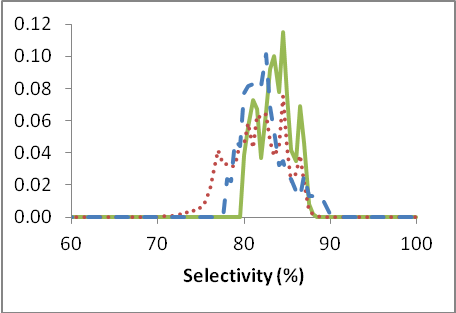
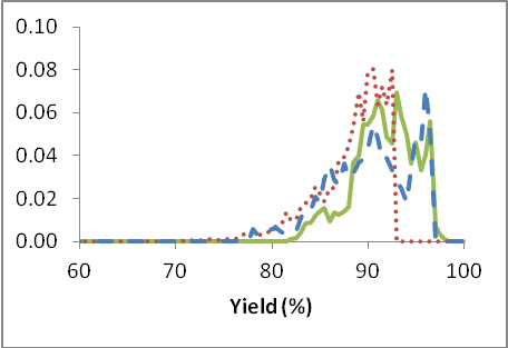
Figure 2: The probability distribution functions for selectivity and yield of Di for periods in which the optimization was not used (reference period: red dotted line), used whenever deemed useful(blue dashed line) and used fully (green solid line).
It is apparent, from these images alone, that we increase the selectivity and the yield with more use of the optimization and that we decrease the variance (i.e. the spreading out or distribution of the results) of both selectivity and yield as well. Decreasing the variance is desirable because it yields a more stable reaction over the long term and thus produces its output more uniformly over time. Numerically, the results are displayed in table 1 below.
Table 1: For both selectivity and yield, we compute the mean ± the standard deviation for all three periods.
The results show that the selectivity can be increased by approximately 2.9% and the yield by approximately 5.1% absolute by comparing the usage with the reference period. Together these two factors yield an increase in profitability of approximately 6% in the plant.
It is to be emphasized that this profitability increase of 6% was made possible through a change of operator behavior only (as assisted by the computational optimization) and no capital expenditures were necessary.
The practical setup of this optimization took approximately two days of time for the operating personnel. The computation time for the computer to construct the necessary functions was about one month. The computer interfaces for input and output of the data are standardized in the industry and can thus be applied readily without delay.
Thus, within about one month, the model can be fully operational without occupying the operators for much time. The approach is thus practicable in a real industrial plant.


